Random effects model

In statistics, a random effect(s) model, also called a variance components model is a kind of hierarchical linear model. It assumes that the dataset being analysed consists of a hierarchy of different populations whose differences relate to that hierarchy. In econometrics, random effects models are used in the analysis of hierarchical or panel data when one assumes no fixed effects (i.e. no individual effects). The fixed effects model is a special case of the random effects model. Note that this is not the case in biostatistics, where the econometric definition of the fixed effects model encompasses what biostatisticians call both the "fixed" and "random" effects.

1 Simple example
2 Variance components
3 Unbiasedness
4 See also
5 References
6 Bibliography

Simple example

Suppose m large elementary schools are chosen randomly from among thousands in a large country. Suppose also that n pupils of the same age are chosen randomly at each selected school. Their scores on a standard aptitude test are ascertained. Let Y_ij be the score of the jth pupil at the ith school. A simple way to model the relationships of these quantities is

$Y_{ij} = \mu %2B U_i %2B W_{ij},\,$

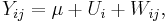
where μ is the average test score for the entire population. In this model U_i is the school-specific random effect: it measures the difference between the average score at school i and the average score in the entire country and it is "random" because the school has been randomly selected from a larger population of schools. The term, W_ij is the individual-specific error. That is, it is the deviation of the j-th pupil’s score from the average for the i-th school. Again this is regarded as random because of the random selection of pupils within the school, even though it is a fixed quantity for any given pupil.

The model can be augmented by including additional explanatory variables, which would capture differences in scores among different groups. For example:

$Y_{ij} = \mu %2B \beta_1 \mathrm{Sex}_{ij} %2B \beta_2 \mathrm{Race}_{ij} %2B \beta_3 \mathrm{ParentsEduc}_{ij} %2B U_i %2B W_{ij},\,$

where Sex_ij is the dummy variable for boys/girls, Race_ij is the dummy variable for white/black pupils, and ParentsEduc_ij records the average education level of child’s parents. This is a mixed model, not a purely random effects model.

Variance components

The variance of Y_ij is the sum of the variances τ² and σ² of U_i and W_ij respectively.

Let

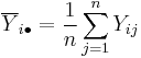
$\overline{Y}_{i\bullet} = \frac{1}{n}\sum_{j=1}^n Y_{ij}$

be the average, not of all scores at the ith school, but of those at the ith school that are included in the random sample. Let

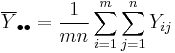
$\overline{Y}_{\bullet\bullet} = \frac{1}{mn}\sum_{i=1}^m\sum_{j=1}^n Y_{ij}$

be the "grand average".

Let

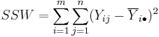
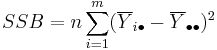
$SSW = \sum_{i=1}^m\sum_{j=1}^n (Y_{ij} - \overline{Y}_{i\bullet})^2 \,$

$SSB = n\sum_{i=1}^m (\overline{Y}_{i\bullet} - \overline{Y}_{\bullet\bullet})^2 \,$

be respectively the sum of squares due to differences within groups and the sum of squares due to difference between groups. Then it can be shown that

$\frac{1}{m(n - 1)}E(SSW) = \sigma^2$

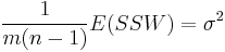
and

$\frac{1}{(m - 1)n}E(SSB) = \frac{\sigma^2}{n} %2B \tau^2.$

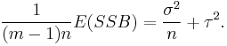
These "expected mean squares" can be used as the basis for estimation of the "variance components" σ² and τ².

Unbiasedness

In general, random effects is efficient, and should be used (over fixed effects) if the assumptions underlying it are believed to be satisfied. For RE to work in the school example it is necessary that the school-specific effects be orthogonal to the other covariates of the model. This can be tested by running random effects, then fixed effects, and doing a Hausman specification test. If the test rejects, then random effects is biased and fixed effects is the correct estimation procedure.

References

Bibliography

Christensen, Ronald (2002). Plane Answers to Complex Questions: The Theory of Linear Models (Third ed.). New York: Springer. ISBN 0-387-95361-2.